Introduction
The double pendulum, an iconic example of chaotic motion, captivates our engineering imagination with its unpredictable behaviour. It is a system comprising two single pendulums in tandem, and it challenges us engineers, physicists, and mathematicians to analyse its intricate dynamics.
In this series of blog posts, we will discuss the simulation of a double pendulum's motion by starting with the derivation of the equations of motion using the Lagrangian approach. This approach provides an elegant and systematic method to understand the motion of mechanical systems, particularly those with constraints and complex geometries.
The series is divided into three parts:
- Introduction & derivation of the Equations of Motion (EOMs)
- Implementation of the derived equations in MATLAB
- Visualisation and animation of relevant quantities inside of MATLAB

With the meme out of the way, let's get into it.
Why Lagrangian Mechanics?
Lagrangian mechanics is often a superior choice for analysing complex mechanical systems like the double pendulum for several reasons:
- Generalised Coordinates: It allows us to use generalised coordinates (\(\theta_1\) and \(\theta_2\)) that describe the system's configuration. This simplifies the analysis by reducing the number of variables compared to Cartesian coordinates.
The system we are investigating looks as follows

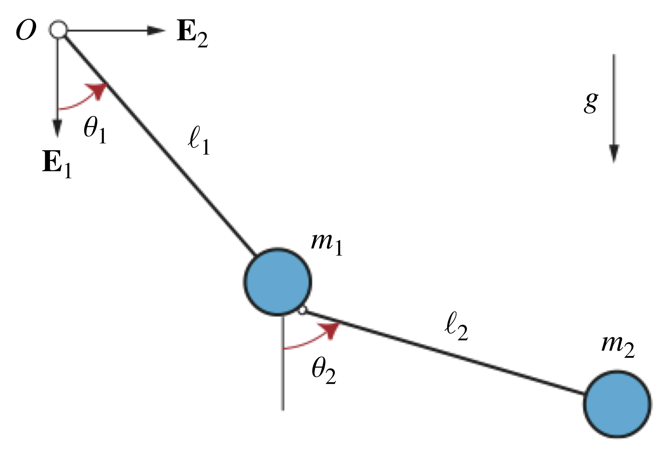
In classical mechanics, when dealing with complex systems, we often encounter multiple physical coordinates (e.g., Cartesian coordinates like x, y, and z) to describe the positions of various parts of the system. However, generalized coordinates offer a more elegant and compact way to represent the system's configuration.
Key characteristics of generalised coordinates:
- Reduced Number: Generalised coordinates reduce the number of variables needed to describe a system. For instance, in a multi-particle system, you might have many physical coordinates, but generalised coordinates provide a minimal set to describe the system.
- Independent Variables: Generalised coordinates are chosen to be independent of each other, which simplifies the mathematical analysis.
- Natural to the Problem: The choice of generalised coordinates should be natural to the problem at hand. They are typically selected to represent degrees of freedom or parameters that uniquely specify the system's configuration.
- No Need for Constraints: Lagrangian mechanics handles systems with constraints naturally. In the case of the double pendulum, there is a constraint due to the fixed length of the rods, and Lagrangian mechanics can handle this constraint without the need for additional equations.
- Elegance and Simplicity: Lagrangian mechanics provides a more elegant and compact formulation of the equations of motion. It allows us to express the system's dynamics in terms of the Lagrangian (L), which is the difference between kinetic and potential energy.
- Derivation of Equations: By applying Lagrange's equations, we obtain a set of second-order differential equations that govern the system's motion directly. These equations are often easier to work with and require fewer computations than the equivalent approach using Newton's laws.
- Conservation Laws: Lagrangian mechanics often reveal conservation laws, such as the conservation of angular momentum and energy, which can be valuable in understanding the system's behaviour.
Another important point that we have to make is that you cannot easily use the small angle approximation. This approximation is a simplifying assumption often used in physics to make the analysis of certain systems, like simple pendulums, easier.
However, it cannot be applied to a double pendulum because the system is highly nonlinear and chaotic. Below are a few reasons:
- Nonlinearity: In a simple pendulum, the restoring force (the force that brings the pendulum back to its equilibrium position) is directly proportional to the angle the pendulum makes with the vertical. This allows us to use a small angle approximation (sinθ ≈ θ for small angles) to simplify the equations of motion. However, in a double pendulum, the restoring forces are not linearly proportional to the angles, which leads to highly nonlinear equations of motion. The small angle approximation, which assumes linearity, is not valid in this case.
- Chaos: A double pendulum is a chaotic system, meaning it is highly sensitive to initial conditions. Even small changes in the initial positions or velocities of the pendulum can lead to dramatically different trajectories. This chaotic behaviour is a result of the complex, nonlinear interactions between the two pendulum arms. The small angle approximation assumes that deviations from the vertical are small and that the system behaves linearly, which is not the case for a double pendulum.
- Complex dynamics: The motion of a double pendulum involves multiple coupled differential equations that are difficult to solve analytically. These equations cannot be easily reduced to a linear approximation like in the case of a simple pendulum.
Therefore, it is best to model the pendulum using Lagrangian mechanics. This is an essential tool in physics that switches us from looking at the forces in a system to looking at the energy in a system. We are switching our frame of reference from deriving forces and including constraints by using kinetic and potential energy.
Step 1 - Define the Lagrangian
The Lagrangian, denoted as L, serves as the foundation of the Lagrangian approach. It is defined as the difference between the kinetic energy (T) and potential energy (V) of the system. This seemingly simple expression encapsulates the essence of the system's dynamics.
The Lagrangian (L) for the double pendulum is defined as:
\begin{equation} L = T - V \end{equation}
Where:
- T is the kinetic energy.
- V is the potential energy.
Step 2 - Derive the Kinetic Energy (T)
To accurately model the double pendulum's motion, we must first grasp its kinetic energy (T). T is calculated as the sum of the kinetic energies of the individual pendulum bobs. By utilising the expressions for velocity in terms of angular variables, we can express T as a combination of the rotational kinetic energies of the two pendulum arms and the translational kinetic energy of the bobs.
In the context of a pendulum, a "bob" refers to the mass at the end of the pendulum's arm. The bob is the part of the pendulum that swings back and forth. It's typically a dense, often spherical, or cylindrical object that provides the mass needed for the pendulum to exhibit its characteristic oscillatory motion. The motion of a pendulum, including its period and frequency, is influenced by the length of the pendulum arm and the mass of the bob. Bobs can vary in size and shape depending on the specific pendulum system and its intended use.
Let's start simple and transform the words into formulas.
The kinetic energy T can be expressed as:
\begin{equation} T = \frac{1}{2} m_1 v_1^2 + \frac{1}{2} m_2 v_2^2 \end{equation}
Where:
- \(m_1\) and \(m_2\) are the masses of the two pendulum bobs.
- \(v_1\) and \(v_2\) are the velocities of the two pendulum bobs.
Using the expressions for velocity in terms of angular variables:
\begin{equation} v_1 = l_1 \dot{\theta}_1 \end{equation}
\begin{equation} v_2 = \sqrt{l_1^2 \dot\theta_1^2 + l_2^2 \dot\theta_2^2 + 2l_1 l_2 \dot\theta_1 \dot\theta_2 cos(\theta_1 - \theta_2)} \end{equation}
Before we put that into T for the kinetic energy, let's spend some time to properly derive the equation \(v_2\).
For the velocity of the second pendulum in a double pendulum system, we can use the expressions for velocity in terms of angular variables.
Here's a step-by-step derivation in 10 steps:
1. First, define the angular velocity \(\dot\theta_1\) and \(\dot\theta_2\) for the first and second pendulums, respectively:
- \(\dot\theta_1\) - Angular velocity of the first pendulum.
- \(\dot\theta_2\) - Angular velocity of the second pendulum.
2. The velocity \(v_1\) of the first pendulum is given by: \(v_1 = l_1 \cdot \dot\theta_1\)
3. To find the velocity \(v_2\) of the second pendulum, we need to consider the relative velocity between the first and second pendulum. This relative velocity involves components in the direction of the pendulum rods and the direction perpendicular to them.
4. The component of velocity \(v_2\) along the direction of the second pendulum's rod (tangential velocity) is due to the rotation of both pendulums: \(v_{2T} = l_1 \cdot \dot\theta_1 + l_2 \cdot \dot\theta_2 \)
Here, \(l_1\) is the length of the first pendulum, and \(l_2\) is the length of the second pendulum.
5. The component of velocity \(v_2\) perpendicular to the second pendulum's rod (radial velocity) is due to the motion of the second pendulum with respect to the first pendulum. It is given by: \(v_{2R} = -l_1 \cdot \dot\theta_1 \cdot sin(\theta_1 - \theta_2) \)
This component is negative because the motion of the second pendulum is in the opposite direction of the radial vector.
6. Now, you can find the magnitude of \(v_2\) by using the Pythagorean theorem for the components:
\(v_2 = \sqrt{v_{2T}^2 + v_{2R}^2} \)
\(v_2 = \sqrt{ (l_1 \dot\theta_1 + l_2 \dot\theta_2)^2 + (-l_1 \cdot \dot\theta_1 \cdot sin (\theta_1 - \theta_2))^2 } \)
7. You can simplify this expression further:
\(v_2 = \sqrt{ l_1^2 \cdot \dot\theta_1^2 + l_2^2 \cdot \dot\theta_2^2 + 2l_1 \cdot l_2 \cdot \dot\theta_1 \cdot \dot\theta_2 \cdot cos (\theta_1 - \theta_2) - l_1^2 \cdot \dot\theta_1^2 \cdot sin^2(\theta_1 - \theta_2)} \)
8. Use trigonometric identity to simplify the term involving the sine:
\( sin^2(\theta_1 - \theta_2) = 1 - cos^2(\theta_1 - \theta_2) \)
9. Substitute this back into the equation for \(v_2\):
\(v_2 = \sqrt{ l_1^2 \cdot \dot\theta_1^2 + l_2^2 \cdot \dot\theta_2^2 + 2l_1 \cdot l_2 \cdot \dot\theta_1 \cdot \dot\theta_2 \cdot cos (\theta_1 - \theta_2) - l_1^2 \cdot \dot\theta_1^2 \cdot (1 - cos^2(\theta_1 - \theta_2))} \)
10. Simplify further:
\(v_2 = \sqrt{ l_1^2 \cdot \dot\theta_1^2 + l_2^2 \cdot\dot\theta_2^2 + 2l_1 \cdot l_2 \cdot \dot\theta_1 \cdot \dot\theta_2 cos (\theta_1 - \theta_2) - l_1^2 \cdot \dot\theta_1^2 \cdot cos^2(\theta_1 - \theta_2)} \)
This is the expression for the velocity \(v_2\) of the second pendulum in terms of the angular variables \(\dot\theta_1\) and \(\dot\theta_2\), and the lengths \(l_1\) and \(l_2\), and the angle difference \(\theta_1 - \theta_2\).
...so with all of the preliminary skirmishing, let's now plug equations 3 and 4 into expression 2.
\begin{equation} T = \frac{1}{2} m_1 (l_1 \dot\theta_1)^2 + \frac{1}{2} m_2 (l_1^2 \dot\theta_1^2 + l_2^2 \dot\theta_2^2 + 2l_1 l_2 \dot\theta_1 \dot\theta_2 cos (\theta_1 - \theta_2)) \end{equation}
Step 3 - Derive the Potential Energy V
The potential energy (V) in the system is linked to gravitational forces. For the double pendulum, we consider the heights of the bobs above a reference level. By employing trigonometric relationships, we derive V, which embodies the potential energy due to the gravitational field acting on each pendulum bob.
\begin{equation} V = -m_1 g y_1 - m_2 g y_2 \end{equation}
Where:
- g is the acceleration due to gravity.
- \(y_1\) and \(y_2\) are the heights of the two pendulum bobs above a reference level.
Using trigonometry:
\begin{equation} y_1 = -l_1 cos(\theta_1) \end{equation}
\begin{equation} y_2 = -(l_1 cos(\theta_1) + l_2 cos(\theta_2)) \end{equation}
So, V becomes:
\begin{equation} V = -m_1 g l_1 cos(\theta_1) - m_2 g (l_1 cos(\theta_1) + l_2 cos(\theta_2)) \end{equation}
Step 4 - Calculate the Lagrangian
With T and V calculated, we can proceed to calculate the Lagrangian (L). L emerges as a function of the generalised coordinates \(\theta_1\) and \(\theta_2\), their derivatives, and the system's parameters.
The Lagrangian succinctly encapsulates the physics of the double pendulum, expressing how kinetic and potential energy interplay to drive the system's motion.
Let's recall the Lagrangian again.
\begin{equation} L = T - V \end{equation}
Plugging everything into the equation yields:
\begin{equation} \begin{array}{l} L = \frac{1}{2} m_1 (l_1 \dot\theta_1)^2 + \frac{1}{2} m_2 (l_1^2 \dot\theta_1^2 + l_2^2 \dot\theta_2^2 + 2l_1 l_2 \dot\theta_1 \dot\theta_2 cos (\theta_1 - \theta_2)) \\ + m_1 g l_1 cos(\theta_1) + m_2 g (l_1 cos(\theta_1) + l_2 cos(\theta_2)) \end{array} \end{equation}
which is the Lagrangian for the double pendulum.
Step 5 - Derive the Equations of Motion Using Lagrange's Equations
Lagrange's equations, the heart of the Lagrangian approach, guide us in deriving the equations of motion. These equations are second-order differential equations that describe the motion of a mechanical system.
For the double pendulum, we have two generalised coordinates: \(\theta_1\) and \(\theta_2\). We apply Lagrange's equations to derive equations of motion that govern the evolution of these coordinates over time. The complexity of these equations arises from the interplay of the masses, gravity, and the geometric arrangement of the pendulum arms.
Lagrange's equations are a fundamental tool in Lagrangian mechanics, and they take the following form:
\begin{equation} \frac{d}{dt} \left( \frac{\partial L}{\partial \dot{q}_i} \right) - \frac{\partial L}{\partial q_i} = 0 \end{equation}
where:
- \(\frac{d}{dt} \) represents the derivative with respect to time.
- L is the Lagrangian, which is a function of generalized coordinates (\(q_i\)), their time derivatives (\(\dot{q}_i \)), and time (t).
- \(\frac{\partial L}{\partial \dot{q}_i}\) represents the partial derivative of the Lagrangian with respect to the time derivative of the i-th generalised coordinate.
- \(\frac{\partial L}{\partial {q}_i}\) represents the partial derivative of the Lagrangian with respect to the i-th generalised coordinate.
In our case of the pendulum, you could simply adapt the generalised coordinate from \( q \) to \( \theta \).
\begin{equation} \frac{d}{dt} \left( \frac{\partial L}{\partial \dot{\theta}_i} \right) - \frac{\partial L}{\partial \theta_i} = 0 \end{equation}
Step 6 - Derive Equations of Motion for \(\theta_1\) and \(\theta_2\)
Applying Lagrange's equations, we derive two equations that specifically govern the motion of \(\theta_1\) and \(\theta_2\) in the double pendulum system.
These equations encapsulate the effects of mass, gravity, and the geometric configuration of the pendulum arms. It is within these equations that the richness and unpredictability of the double pendulum's behaviour are encoded.
Solving them analytically is often challenging, leading us to numerical simulations as a means of exploring the system's dynamics. This is exactly what we will do in the second part of this double pendulum blog series.
Calculating the terms needed for the Lagrange equation for \(\theta_1\)
\begin{equation} \frac{\partial L}{\partial \dot\theta_1} = (m_1 + m_2)l_1^2 \dot\theta_1 + m_2 l_1 l_2 \dot\theta_2 cos(\theta_2 - \theta_1) \end{equation}
\begin{equation} \begin{array}{l} \frac{d}{dt} \frac{\partial L}{\partial \dot\theta_1} = (m_1 + m_2)l_1^2 \ddot\theta_1 + m_2 l_1 l_2 \ddot\theta_2 cos(\theta_2 - \theta_1) \\ -m_2 l_1 l_2 \dot\theta_2 sin(\theta_2 - \theta_1) + m_2 l_1 l_2 \dot\theta_1 \dot\theta_2 sin(\theta_2 - \theta_1) \end{array} \end{equation}
\begin{equation} \frac{\partial L}{\partial \theta_1} = m_2 l_1 l_2 \dot\theta_1 \dot\theta_2 sin(\theta_2 - \theta_1) - (m_1 + m_2) g l_1 sin \theta_1 \end{equation}
The Lagrange equation for \( \theta_1 \) is then
\begin{equation} \begin{array}{l} 0 = \frac{d}{dt} \frac{\partial L}{\partial \dot{\theta}_1} - \frac{\partial L}{\partial \theta_1} \\ = (m_1 + m_2) l_1^2 \ddot\theta_1 + m_2 l_1 l_2 \ddot\theta_2 cos(\theta_2 - \theta_1) \\ -m_2 l_1 l_2 \dot\theta_2^2 sin(\theta_2 - \theta_1) + (m_1 + m_2) g l_1 sin \theta_1 \end{array} \end{equation}
Calculating the terms needed for the Lagrange equation for \(\theta_2\)
\begin{equation} \frac{\partial L}{\partial \dot\theta_2} = m_2 l_2^2 \dot\theta_2 + m_2 l_1 l_2 \dot\theta_1 cos(\theta_2 - \theta_1) \end{equation}
\begin{equation} \begin{array}{l} \frac{d}{dt} \frac{\partial L}{\partial \dot\theta_2} = m_2 l_2^2 \ddot\theta_2 + m_2 l_1 l_2 \ddot\theta_1 cos(\theta_2 - \theta_1) \\ +m_2 l_1 l_2 \dot\theta_1 sin(\theta_2 - \theta_1) - m_2 l_1 l_2 \dot\theta_1 \dot\theta_2 sin(\theta_2 - \theta_1) \end{array} \end{equation}
\begin{equation} \frac{\partial L}{\partial \theta_2} = -m_2 l_1 l_2 \dot\theta_1 \dot\theta_2 sin(\theta_2 - \theta_1) - m_2 g l_2 sin \theta_2 \end{equation}
The Lagrange equation for \( \theta_2 \) is then
\begin{equation} \begin{array}{l} 0 = \frac{d}{dt} \frac{\partial L}{\partial \dot{\theta}_2} - \frac{\partial L}{\partial \theta_2} \\ = m_2 l_2^2 \ddot\theta_2 + m_2 l_1 l_2 \ddot\theta_1 cos(\theta_2 - \theta_1) \\ +m_2 l_1 l_2 \dot\theta_1^2 sin(\theta_2 - \theta_1) + m_2 g l_2 sin \theta_2 \end{array} \end{equation}
Implementation in MATLAB
To translate these theoretical concepts into action, we can now use the derived formulas and implement the equations of motion in MATLAB. This allows us to not only simulate the double pendulum's motion but also visualise its behaviour. In the code, we define the system's parameters and initial conditions, compute the Lagrangian, and set up a function suitable for use with MATLAB's ODE solvers. This combination of theoretical understanding and numerical simulation provides a comprehensive view of the double pendulum's dynamics.
Implementing the entire process of solving the equations of motion for a double pendulum in MATLAB can be a complex task, and the code can become quite extensive.
In the next blog, I will showcase the code for a double pendulum. Please note that due to the complexity of the problem, a full implementation will require a bit more than 3-4 lines of code and will involve numerical solvers for differential equations.
Conclusion
So far, we've delved into the Lagrangian approach, a powerful framework for analysing mechanical systems. The approach provides an elegant solution to understanding complex systems with constraints and non-conservative forces.
Simulating the double pendulum's motion reveals the system's chaotic and unpredictable nature, making it not just a mathematical challenge but also a captivating illustration of classical mechanics.
If you're eager to explore further, you can check out the MATLAB code to experiment with different initial conditions and parameters in the next blog. The double pendulum, as a classical problem, not only demonstrates the beauty and intricacy of physics but also serves as a reminder of the profound interplay between mathematics and the natural world.
The secrets of the double pendulum are a testament to the power of Lagrangian mechanics and the excitement of exploring the complexities hidden within the seemingly simple. As we wrap up our journey, we encourage you to experiment with the code and continue your exploration of the captivating world of classical mechanics.
If this post was helpful to you, consider subscribing to receive the latest blog updates! 🙂
And if you would love to see more on MATLAB & engineering, please comment under this post!👇
Keep engineering your mind! ❤️
Jousef