Introduction

If you haven’t been hiding under a stone during your engineering studies, you should have heard about the Finite Element Method (FEM). And maybe you even learned some of its practical aspects by playing around with software packages such as ANSYS, ABAQUS or SimScale.

In this blog, I am going to introduce the Finite Element Method without any heavy mathematical explanations and it is by no means a course on FEM - this is reserved for future posts.

Generally speaking, the finite element method (FEM) is a numerical method used to perform a finite element analysis (FEA) of any given physical phenomenon to predict the behaviour of a structure.

What is the Finite Element Method? 🤔

For the vast majority of geometries and problems, Partial Differential Equations cannot be solved with analytical approaches. Instead, we can approximate these equations using discretisation methods that can be solved using numerical methods.

Therefore, the solutions we get are also an approximation of the real solution to those PDEs. The FEM is such an approximation method that subdivides a complex space or domain into a number of small, countable, and finite amount of pieces (thus the name finite elements) whose behaviour can be described with comparatively simple equations.

The method was originally developed for engineering analysis to model and analyse complex systems in mechanical, civil, and aeronautical engineering. The basics of the method can be derived from Newton's laws of motion, conservation of mass and energy, and the laws of thermodynamics.

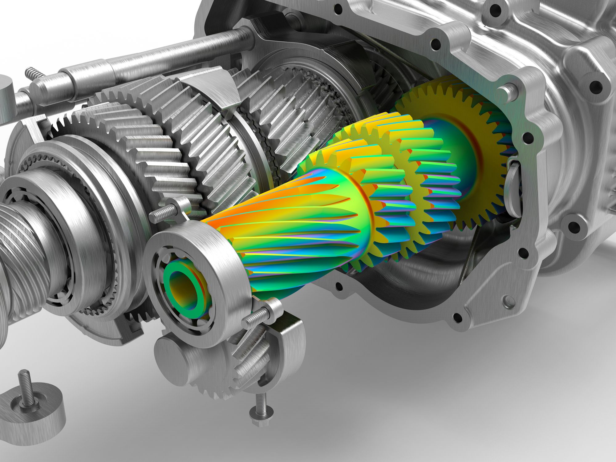
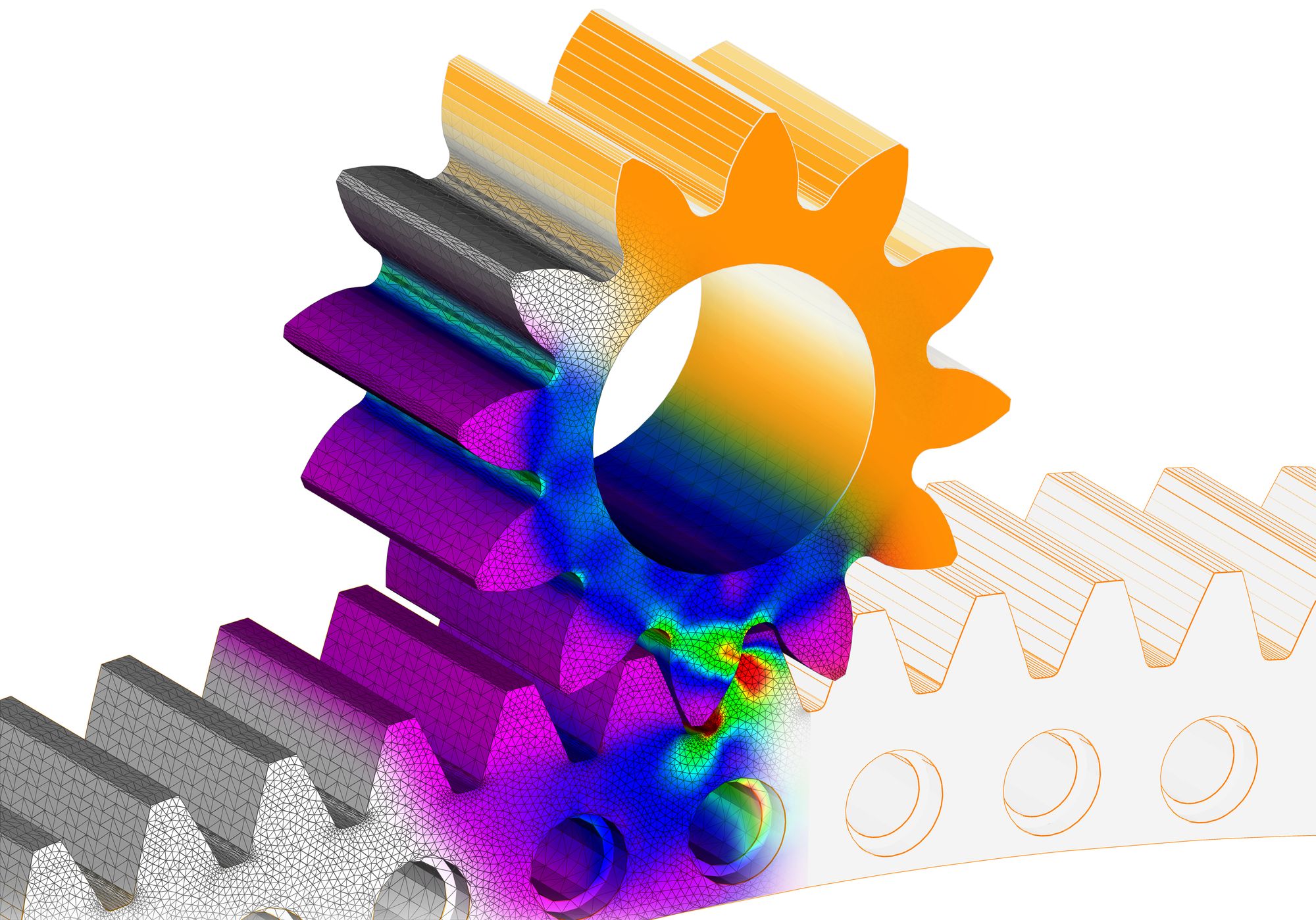
FEM can be used, for example, to determine the structural mechanics of different parts of a car under different loading conditions, the heat flow through engine part, or the distribution of electromagnetic radiation from an antenna.

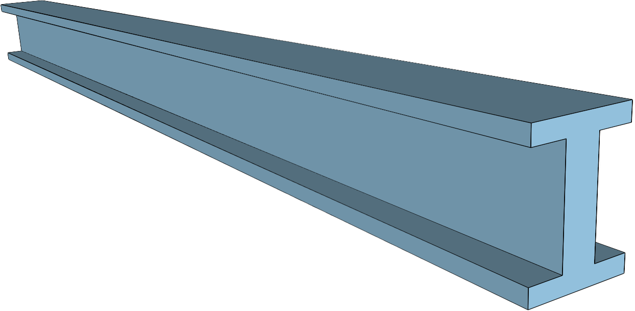
An important aspect of FEM is how the Computer-aided design (CAD) model is prepared for the analysis and is being subdivided during meshing (discretisation into smaller elements).

CAD software such as Creo can be used to define 3D shapes of an object and then imported into a separate FEA tool which subdivides the object into appropriately sized elements according to the desired boundary conditions or mesh.

History & Background 📜

• The term Finite Element was introduced 1960 by Ray William Clough  in his paper "The Finite Element Method in Plane Stress Analysis". In the early 60s this method has been used by several engineers for stress analysis, fluid transport, heat transport and other subjects
• The first Finite-Element-Method book has been published by Olgierd Zienkiewicz, Richard Lawrence Taylor and Jianzhong Zhu
• In the late 60s and 70s the field of FEM application expanded and became a leading numerical approximation in a broad field of engineering problems
• Most commercial codes like ANSYS, ABAQUS, Adina and several others have their origin in the 1970s
• John Swanson releases the first version of his so-called ANalysis SYStems (ANSYS) FEA software tool (1970)
• A web search (2006) for ‘finite element’ using Google yielded over 14 million pages compared to 2022 with 128 million pages
• The number of papers have gone from one (1956) to more than a million (2022)
• FEM systems at Mercedes in the early beginnings have been solved using punchcards (see video below)

A 15 minute introduction to the FEM in German👇

Motivation 💪

Engineers use the finite element method for several good reasons. One of them being is that analytical models are limited in their application. This is the case if we have:

• complex geometries or deformation (e.g. crash testing)
• complex loadings (e.g. time dependent force application)
• complex material laws such as:

1. Anisotropic material law (fibre-reinforced plastic or crystalline material)
2. Inhomogeneous material properties (Young’s modulus…)
3. Hyperelastic material

and many more...

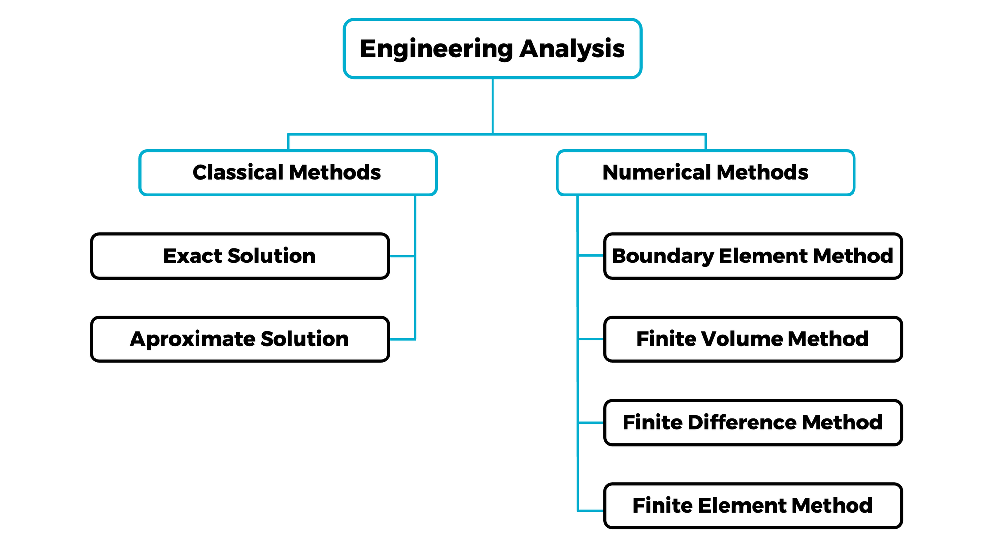
Numerical Methods 🧮

In general, there are three methods on how engineers are able to solve engineering problems.

1. Classical Methods
2. Numerical Methods
3. Experimental Methods

Whenever engineers solve complex problems involving complex geometries, loading conditions or material laws, they cannot use classical analytical approaches using closed-form methods. Therefore numerical methods offer a way to solve a problem where an analytical solution does not exist!

A closed form solution is an expression for an exact solution given with a finite amount of data.

Partial Differential Equations (PDEs) 📝

The description of nature and the laws of physics for space- and time-dependent problems are usually expressed with partial differential equations (PDEs). These equations are solved in an approximate manner by the finite element method (FEM) which is based on equations of classical methods such as the Theory of Elasticity.

PDEs are equations for an unknown function of two or more independent variables that involves partial derivatives. Below is an example of a PDE, namely the three-dimensional Laplace equation where \[ \phi \] is the dependent variable, and x, y, and z are the spatial independent variables.

\[ \frac{\partial^2 \phi}{\partial x^2} + \frac{\partial^2 \phi}{\partial y^2} + \frac{\partial^2 \phi}{\partial z^2} = 0  \]

In order to solve this equation, it must be subjected to so-called initial conditions and boundary conditions.

An Initial Boundary Value Problem (IBVP) consists of the Partial Differential Equation the Initial Conditions as well as the Boundary Conditions

👉 Initial Boundary Value Problem = PDE + ICs + BCs

Other examples of famous PDEs are:

• Navier-Stokes Equations
• Schrödinger's Equation
• Heat Equation
• Maxwell's Equations
• Wave Equation

Basic Boundary Conditions in FEA 🧱

Generally speaking, boundary conditions (BCs) are constraints necessary for the solution of a boundary value problem.

A boundary value problem is a differential equation (or system of differential equations) to be solved in a domain on whose boundary a set of conditions is known. Compared to the "initial value problem", in which only the conditions on one extreme of the interval are known. Boundary value problems are extremely important as they model a vast amount of phenomena and applications, from solid mechanics to heat transfer, from fluid mechanics to acoustic diffusion. They arise naturally in every problem based on a differential equation to be solved in space, while initial value problems usually refer to problems to be solved in time.

Generally speaking, boundary conditions for continuous systems are classified as being of two types.

• Geometric (Essential) Boundary Conditions
• Natural Boundary Conditions

Geometric (Essential) Boundary Conditions 📐

Those BCs also known as Kinematic Boundary Conditions must be satisfied according to geometric constraints. For example:

\[ u(x=0) = 0 \quad \text{\&} \quad u'(x=0) = 0 \]

at a fixed end of a cantilever.

• This boundary condition can be a "fixed BC" in your FEA tool and constraints a shaft and its position in space
• Boundary conditions which are related to the geometry, are called geometric boundary conditions

Force (Natural) Boundary Conditions 💪

Those BCs also known as Static Boundary Conditions must be satisfied as a result of free and moment balances. For example:

\[ EI \frac{\delta^2 u}{\delta x^2}(x = L) = 0 \]

is a moment boundary condition at the free end of a cantilever. So, it is prescribed by forces and moments.

• This is the boundary condition is prescribed as a load acting on your component
• Boundary conditions which are related to loadings, are called force boundary conditions

Approach of the FEM 💻

From a mathematical point of view, the following five steps are essential to know in order to understand how the FEM is working behind the scenes.

Step #1

• Create geometry (CAD Model)
• Define material properties
• Choose initial and boundary conditions
• Define other conditions such as contact behaviour
• Discretisation of the geometry 👉 "Meshing"

Pre-Processing, also called model preparation, is usually the most labor-intensive step of FEA.

Step #2
Element formulation 👉 development of equations for elements
Set up the partial differential equation in its weak form

Step #3
Assembly: Set up global problem 👉 obtaining equations for the entire system from the equations for one element

Step #4
Solving system of linear equations

Step #5
Post-Processing: determining quantities of interest, such as stresses and strains and obtaining visualisations of the response

Hint: The solver may produce impressive, colourful results which may look convincing but can be completely useless. Try to compare your solution with analytical results (if available), perform a proper convergence study and/or compare your results with existing papers / literature.

There are obviously more points to check when validating and correlating your FEA results which will be covered in another post. For now you only have to know not to trust your results and you have to employ methods to go through a meticulous verification and validation process for every analysis.

In the section on FEA Workflow, we will have a look at a more granular level of how FEA works. In practise, you are neither really busy thinking about how the matrix is assembled, nor do you care how the system of equations are solved which is just a bunch of number crunching behind the scenes.

Divide & Conquer 🚀

A characteristic feature of the finite element method is that instead of seeking the approximation over the entire region, the region is divided into smaller parts, so called finite elements and the approximation is then carried out over each element.

The collection of all small parts is called the finite elements.

When the type of approximation has been chosen (is to be applied over each element), the corresponding behaviour of each element can then be determined. Having determined the behaviour of all single elements, the elements can then be patched together (Matrix Assembly), which enables us to get an approximate solution of the entire body over the entire domain.

As we mentioned before, we need to approximate a solution over our elements in order to determine the behaviour. This approximation is usually a polynomial and is, in fact, some interpolation over the element. This means we know some values at certain points within the element but not at every point. These ‘certain points’ are called nodal points and are often located at the boundary of the element. The accuracy with which the variable changes is expressed by the approximation, which can be linear, quadratic, cubic et cetera.

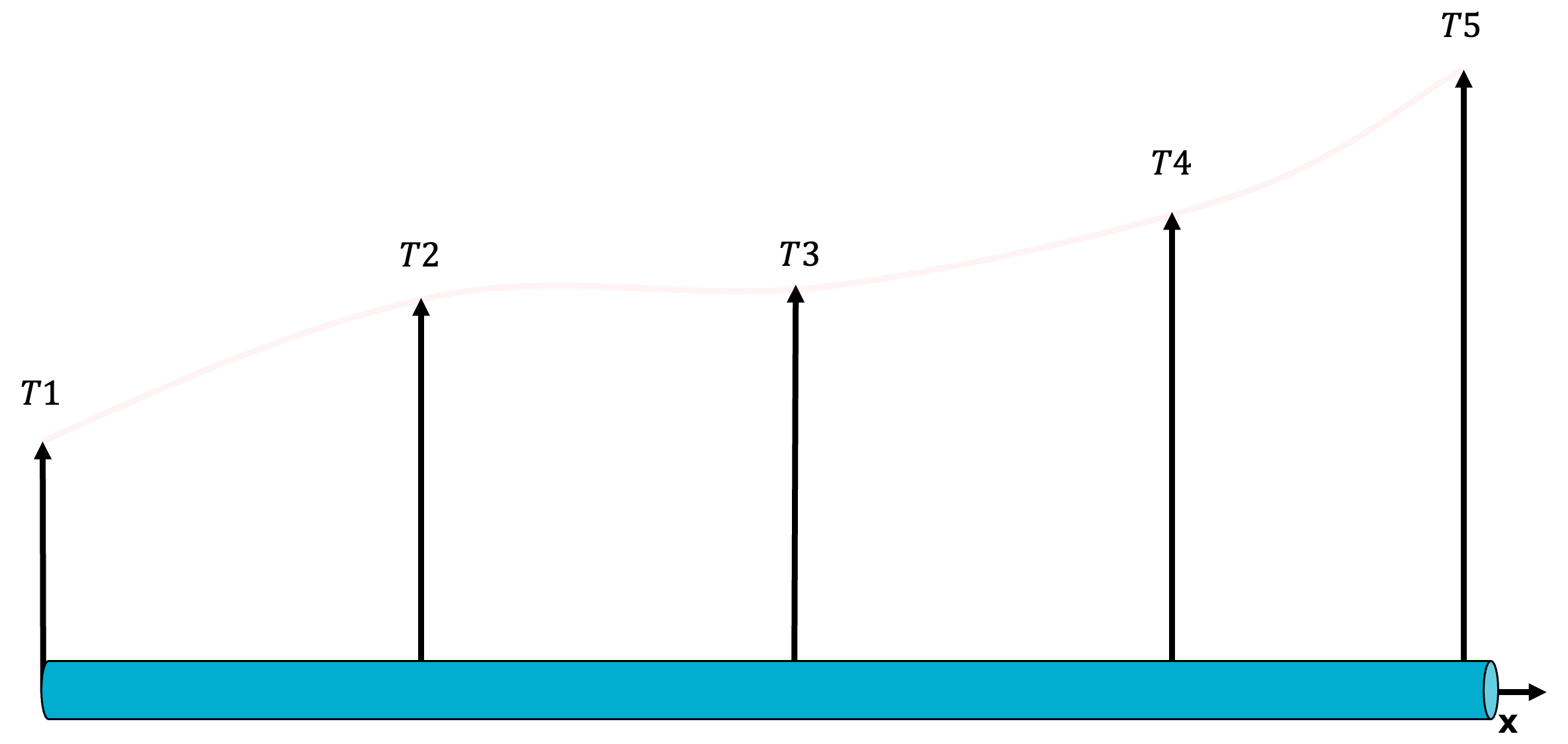
In order to get a better understanding of approximation techniques, we will look at a one-dimensional bar. Consider the true temperature distribution T(x) along the bar in the picture below.

Equidistant grids can waste many nodes in areas where the solution is not important or changes in quantities (gradients) are insignificant.

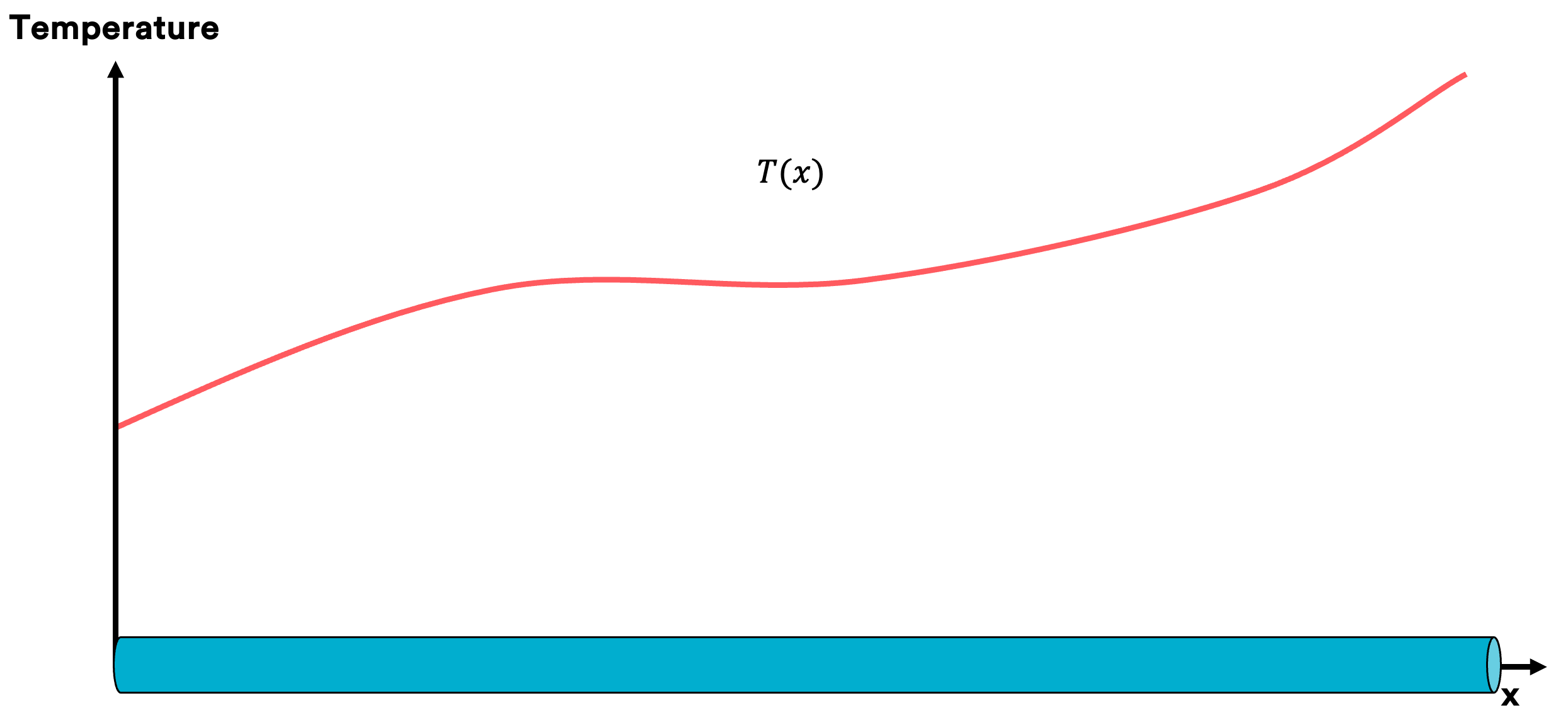
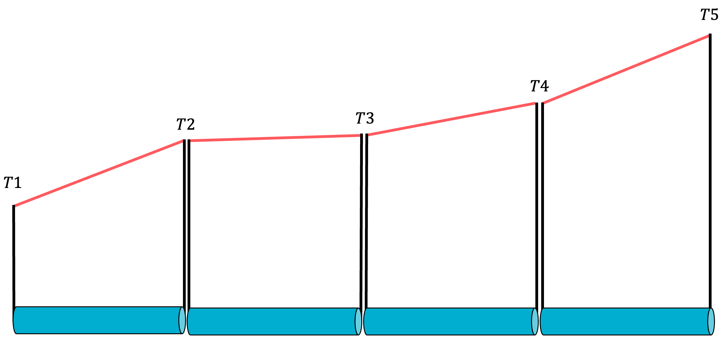
The nodal points we chose do not need to be equally spaced! We now divide our bar into four elements over which the temperature is assumed to vary in a linear manner between each nodal point!

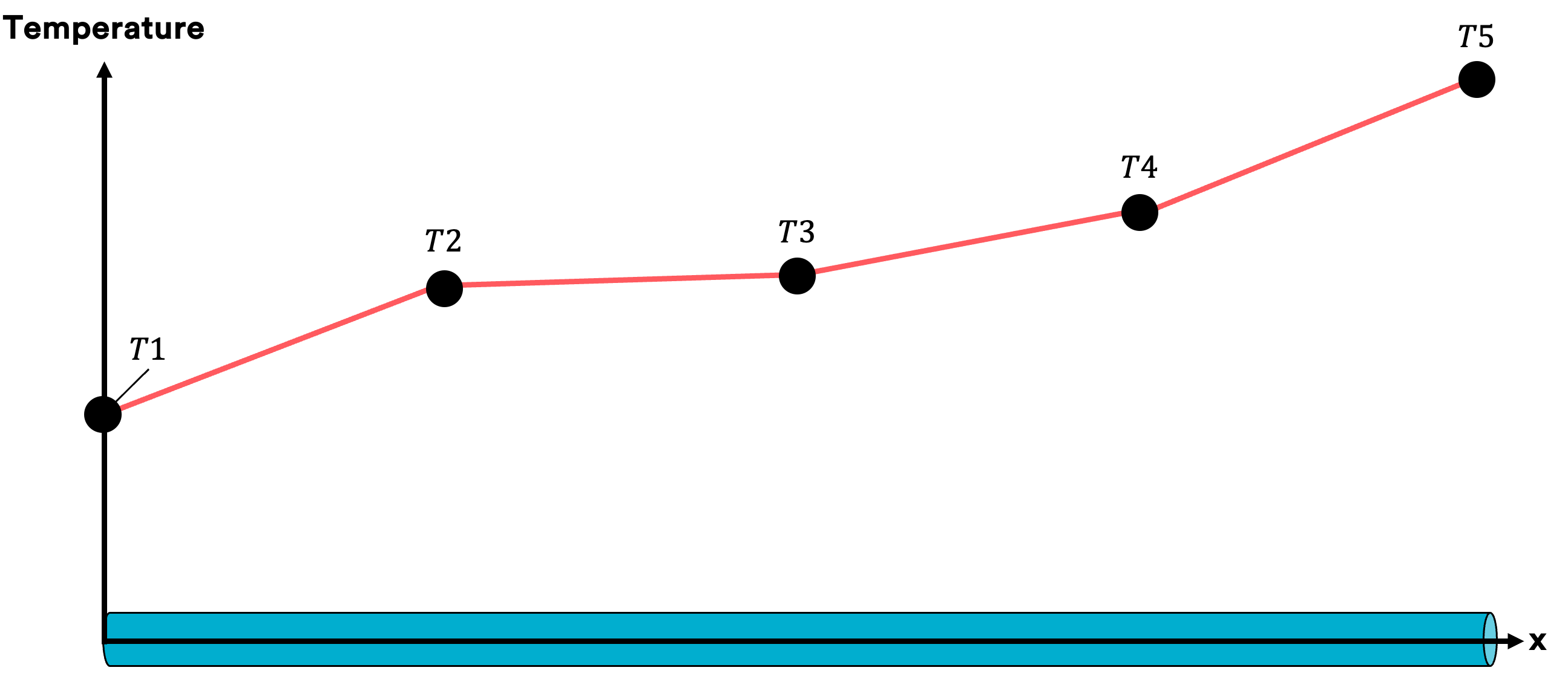
Well we see linear approximation is quite good, but we can certainly do better! If we chose a quadratic approximation the temperature distribution along the bar is way more smooth.

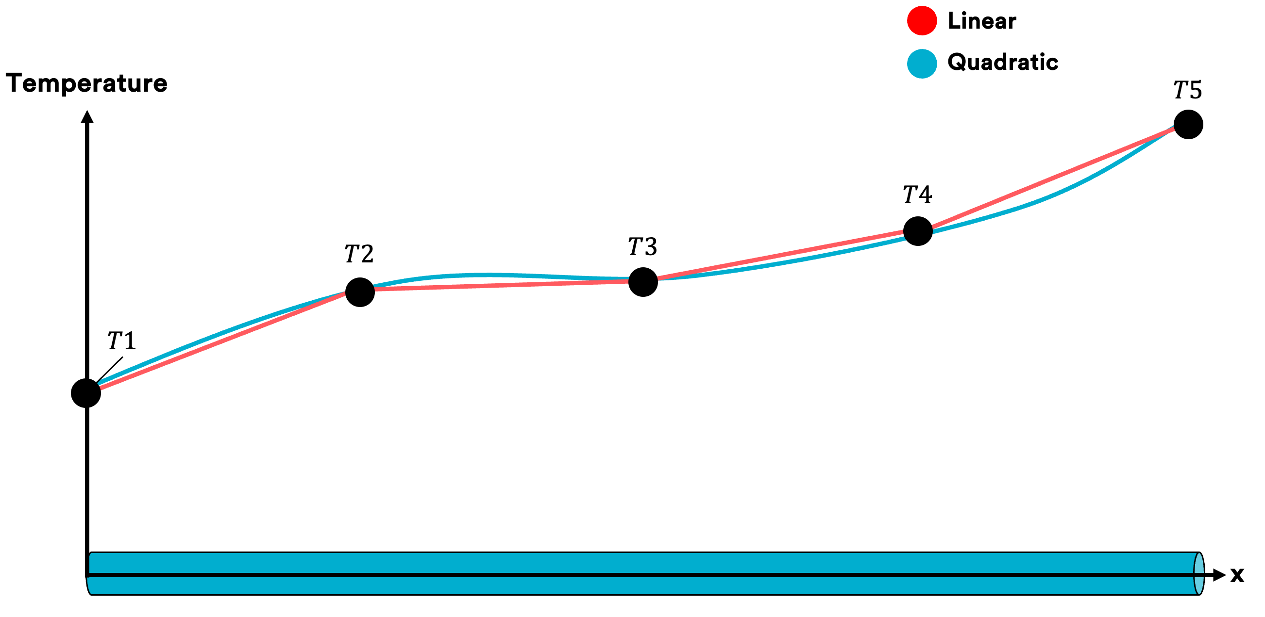
Nevertheless, we see that irrespective of the polynomial degree the distribution over the fin is known once we know the values at the nodal points, simple as that. If we just have one bar we would have an infinite amount of unknowns (Degree of Freedom (DoF)). But in this case we have a problem with a finite number of unknowns.

A system with a finite number of unknowns is called a discrete system

A system with an infinite number of unknowns is called a continuous system

In our case we would have a system consisting of five equations which can be solved by hand but in general we have thousands and thousands of unknowns. Luckily we have powerful machines at our fingertips allowing us to solve such problems for us which makes life way easier.

FEA Workflow 💡

In general, the FEA workflow can be broken down into

1. Pre-Processing
2. Processing
3. Post-Processing

Pre-processing is performed to create the model, generate an appropriate finite element grid, apply the appropriate boundary conditions, and view the total model.

Processing refers to the number crunching part behind the scenes.

Post-processing provides visualisation of the computed results and gives meaning to the hundreds of numbers that could otherwise not be interpreted by any human being.

Part 1 – Geometry 📐

This is the part where you import your CAD model. Ideally, all redundant parts of the part that do not contribute to the analysis or require excessive model setup have been removed

CAD modeling is used by many designers to create elaborate computerized models of objects before they are physically produced.

In general, there are two ways on how to create or import CAD models, depending on which FEA software you're using.

• Directly Import CAD: A very common solution is that your FEA tools allows you to import CAD models. Obviously, this assumes that you already have a model available and modelled in your CAD software (Creo, Solidworks etc.). There are tools such as ABAQUS that allow you to create your geometry inside the tool itself.
• Create CAD Inside the Tool: This is a method that can be used assuming that your tool of choice allows creating a CAD model from scratch.

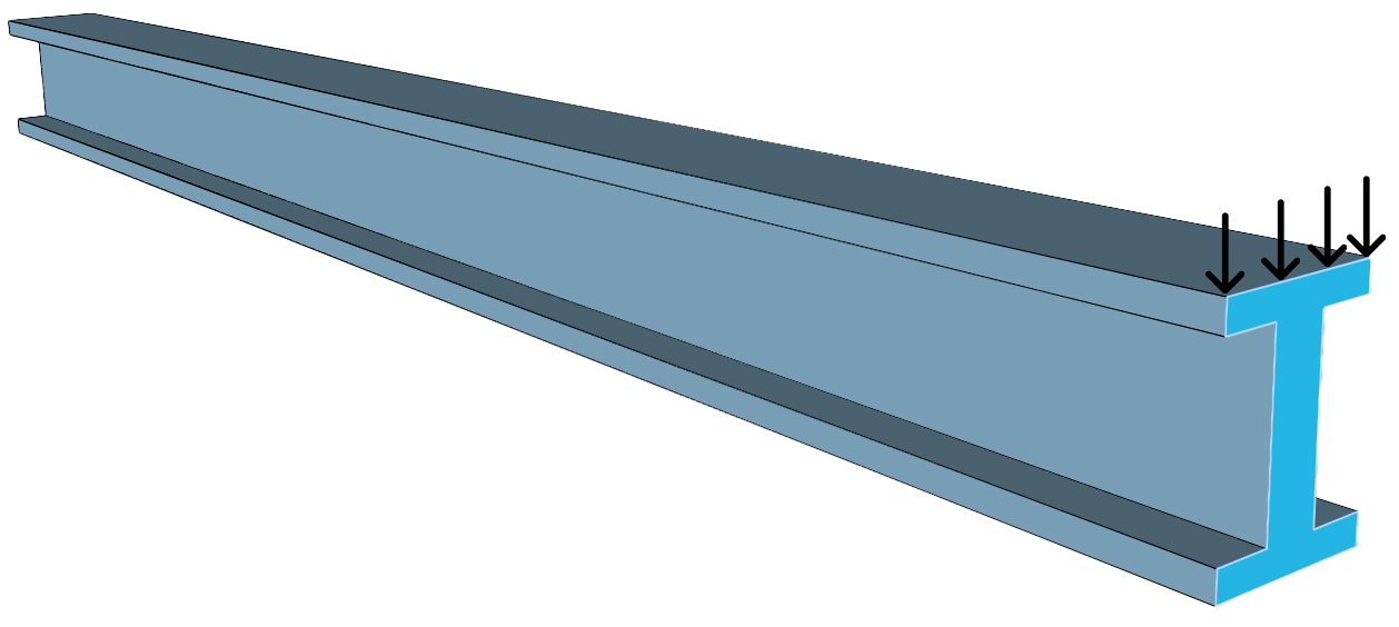
Part 2 – Material & Boundary Conditions 🔗

The definition of material and boundary conditions (BCs) can usually be captured at once .

• Material Definition: In this step, you have to define what material you will be using and define at the very minimum the Young's modulus, the Poisson's ratio and material density. Once the basics are done, you can even decide what material laws shall be applied such as linear elastic behaviour or if the material will have plastic behaviour.

Material nonlinearity involves the nonlinear behaviours of material based on current deformation, temperature, pressure and so on. Some nonlinear material models are large strain, stress-strain relationship, elastoplasticity, plasticity, creep and hyperelasticity.

• Boundary Conditions (BCs): This is one of the most complicated topics in FEA as you have to decide how the real life conditions can be translated into a digital representation without simplifying it too much. Trust me, this is way trickier than you think it is!

As a beginner, you can be quite sure that you will mess up boundary conditions very often as you not only have to understand how BCs can be used in your model but also how the software is treating each BC.

• Loads: Loads can be forces, moments, accelerations or even temperature loads on your components.
• Contacts: Bodies can be connected to each other via common nodes. These connections are only possible if the two bodies have the same mesh at the interface.

Contact is one type of nonlinearity of the system. An abrupt change in stiffness may occur when bodies come into or out of contact with each other. This is a result of the changing nature of the contact between components in the analysis during motion.

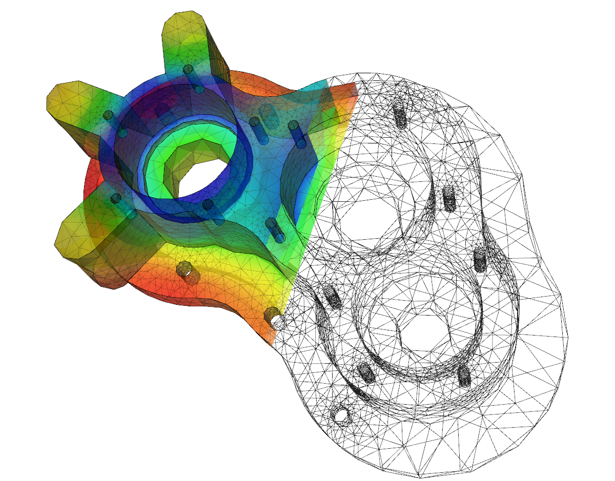
Part 3 – Discretisation ("Meshing") 🖥

Meshing is an interesting but also difficult topic which has many aspects to consider. Personally, CAD cleanup is the most tedious part whereas other engineers will say that meshing is the worst job for them - it's up to you to decide!

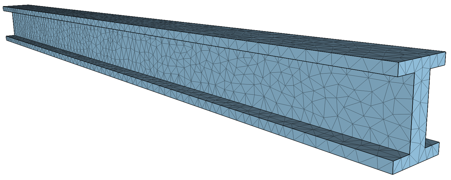
The following questions have to be answered when meshing:

• What element types do I choose? (TET vs. HEX - 1D, 2D or 3D?)
• Do I choose first order elements or second order elements?
• How do I know that my mesh is fine enough? 👉 Convergence Study
• Do I have to mesh finer in certain regions?

Often, critical stresses are limited to small areas of a model. When a global mesh refinement is used, the resulting mesh is often too fine in areas that are not relevant for the evaluation process.

A more efficient approach is to refine the mesh locally where critical stress regions are located. FEA tools often allow you to use Local Mesh Refinements that provide a targeted mesh refinement.

Part 4 – Solving the System of Equations  🖥

The solver is now doing a bunch of number crunching on a system of equations behind the scenes of the FE model. Systems of equations with more than 10 million equations are not uncommon but also not unsolvable considering how fast and efficient modern codes and machines are.

The first result of includes the displacements of the individual nodes. In subsequent steps, distortions, stresses as well as nodal forces can be calculated. In addition to mechanical quantities, thermal, electrical or magnetic quantities can also be calculated if a thermo-mechanical or electromagnetic solver is used.

An equation that you should know about is

\[ \{F\}= [K]\{u\} \]

which is the standard equation for the FEM where

• {F} are the forces acting on the structure
• [K] is the stiffness matrix
• {u} are the displacements

You will see in another blog post, that if we only have a look at a linear spring element to derive the fundamental equation for the FEM, the rows of the stiffness matrix are linearly dependent which means that the system is statically underdetermined!

We have to integrate boundary conditions into the system, otherwise our solver will end up with an error.

Whenever we apply external forces and calculate displacements, this is called a Displacement-based procedure

Whenever we apply displacements and calculate the forces, this is called a Force-based procedure

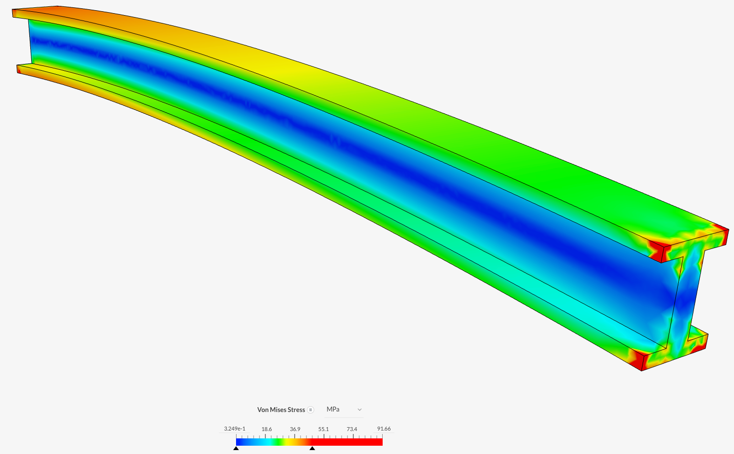
Part 5 – Post-Processing 🎨

Post-Processing is the part where the numbers from the solver are taken and made interpretable for the engineers - otherwise we would have a hard time decoding what all those numbers actually mean.

It is important to know it is not sufficient to simply accept the beautiful images that the machine throws at you. You need to take your engineering knowledge and intuition and really think hard if the results actually make sense and are physically accurate.

GIGO = Garbage In equals Garbage Out

Part 6 – Iteration ↩️

Simple doing one analysis and looking at the plots won't do the job. FEA is an iterative process which requires an engineer to make adaptations to the model, fix boundary conditions and potentially perform several meshes to see if there are no significant changes in stresses or other relevant output quantities the finer we discretise our domain.

If no convergence can be seen, this can be an issue of a so-called singularity.

A finite element model will sometimes contain a so-called singularities which means that there are points in your model where values (such as stresses) tend towards an infinite value.

In the worst case, you have to go back to Step 1 and adapt your CAD model.

FEA Capabilities 🚀

FEA can be applied to different types of single or multiphysics problems involving heat transfer, fluid dynamics, electric fields and more. Three main types of problems are:

• Static: For example, structural analysis of different parts of a building or bridge when a certain load is applied with no motion involved. Knowing what parts experience the highest stress tells the designers what parts need to be strongest
• Dynamic: Useful when the forces applied to the system change over time, for example, heat flow through a system component
• Modal: Useful in analysing the effects of vibration on a system

Over the years, more "exotic" topics in FEA have emerged:

• Extended FEM (XFEM): The word extended is added as the method enhances crack-propagation simulation capability of the conventional finite elements formulation. This method is useful when analysing systems with discontinuities, such as fractures; and answers questions how a system behaves when one or several components have a crack or other defects.
• Generalised FEM (GFEM): Combines traditional mesh-based FEM with more advanced "meshless" methods. It combines the features of the traditional FEM and meshless methods. One of the advantages of GFEM is the prevention of re-meshing around singularities.
• Mixed FEM: Useful for problems involving contact or incompressibility, and where constraints are imposed using Lagrange multipliers. These extra degrees of freedom arising from Lagrange multipliers are solved independently. The system of equations is solved like a coupled system of equations.
• hp-FEM: hp-FEM is a combination of automatic mesh refinement (h-refinement) and an increase in the order of polynomial (p-refinement). It is however not the same as doing h- and p- refinements separately. The method is used when certain elements in a system are further subdivided (in a process called mesh refinement), and the polynomial equations of each element have different orders.
• Discontinuous Galerkin FEM: DG-FEM has shown significant promise for utilising the idea of finite elements to solve hyperbolic equations, where traditional finite element methods have been weak. Used to analyse systems in which components bend and for incompressible problems which are typically observed in most material processes.

Advantages of FEM 📈

1. Modelling of complex geometries and irregular shapes are easier as varieties of finite elements are available for the discretisation of the domain
2. Different types of material properties can be easily accommodated, either from element-to-element or even inside an element
3. Higher order elements may be implemented if the tools allow it
4. FEM is simple, well-defined and result-oriented and widely popular among an enthusiastic engineering community that can help you whenever you run into problems
5. The availability of a large number of FEA software packages and literature makes FEM a versatile and powerful, and accessible numerical method

Disadvantages of FEM 📉

Although FEM is an incredibly powerful method, there are however some drawbacks.

1. Simplification of real life components can’t be 100% exact for complex shapes
2. FEM is an approximate method and engineers are motivated to minimise the error over the whole domain
3. Although FEM is simple from its principles, the mathematics behind the FEM is relatively advanced, and thus requires mathematical expertise for its implementation
4. The computation is very costly in FEM. As your mesh becomes finer, you will need more RAM. Almost all FEM packages use the concept of bandwidth reduction to reduce the amount of memory needed to store the stiffness matrix
5. The time needed for solving a FE problem increases with the degree of fineness of the mesh
6. Proper engineering judgement is needed to interpret results

Finite Element Method - Trends 🚀

Various applications of the FEM prove that this technique is of great value as it provides a means with which engineers can create efficient designs for large and complex problems, which cannot be solved using analytical methods.

The FEA process incorporates many complex steps and involves numerous parameters which can be tweaked by the user. Thanks to the democratisation of FEA, software is much more streamlined, easy to integrate into engineering R&D processes and much more affordable to every engineer, designer and smaller enterprises.

In the future, the use and availability of cloud-enabled services such as SimScale will be intensified during design projects. The past and present of mathematical modelling and FEA software is a success story which will be enhanced using Artificial Intelligence (AI) marking a significant step in FEA history.

Not only will engineers have to do less effort, but the analyses will be more accurate and faster augmenting the whole product development process from conception to prototyping. This allows engineers to be more creative in the design process and focus less on tuning sensitive FE parameters.

The Finite Element Method - A Beginner's Guide 🎬

If that post was helpful to you, consider subscribing to my latest blogs, tutorials and course updates – costs you less than a Starbucks coffee! 😉

And if you would love to see another topic on FEA, please leave a comment!👇

Keep engineering your mind! ❤️

Jousef