Introduction
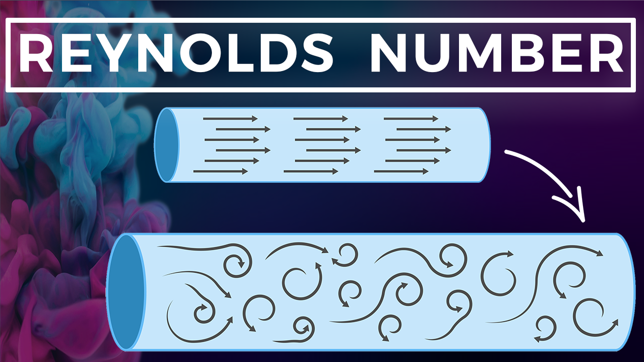
The intricate motion of fluids is incredibly difficult to predict due to its nonlinear nature. As engineers, physicists or biologists, we can luckily predict whether the flow in a given system should be laminar or turbulent, thanks to an Irish genius and physicist named Osborne Reynolds.
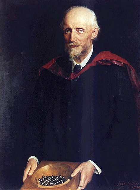
Reynolds was a pioneer in the study of fluid dynamics, performing a simple but elegant experiment to demonstrate that the transition point between the two types of flow could be predicted by one simple number, that we now know as the important and convenient Reynolds number, commonly referred to as Re.
Although the concept was introduced by George Stokes in 1851, Arnold Sommerfeld named the Reynolds number in 1908 after Osborne Reynolds!
In general, the Reynolds Number is defined as the ratio of inertial force to viscous forces and quantifies the relative importance of these two types of forces for given flow conditions - an important concept that we will also cover in this blog post.
To this day, the Reynolds number remains the standard mathematical framework to study laminar & turbulent fluid systems.
Formula & Derivation 💦
The Reynolds number is defined as a characteristic length multiplied by a characteristic velocity and divided by the kinematic viscosity.
\[ Re = \frac{\rho VD}{\mu} = \frac{VD}{\nu} \]
where:
- V is the flow velocity
- D is the characteristic dimension of the object (traveled length of the fluid such as the hydraulic diameter, chord length of an airfoil etc.)
- ρ fluid density (kg/m3)
- μ dynamic viscosity (Pa•s)
- ν kinematic viscosity (m2/s) 👉 ν = μ / ρ
Whenever viscous forces are dominant (slow flow, low Re), they are sufficient enough to keep all the fluid particles in line, then the flow is called laminar. Very low Reynolds Numbers indicate viscous creeping motion, where inertial effects are negligible. When the inertial forces dominate over viscous forces (when the fluid flows faster and Re is larger), the flow is said to be turbulent.
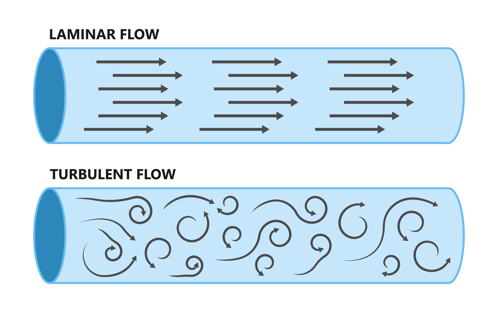
Laminar Flow 💧
Laminar flow is the movement of fluid particles along well-defined paths or streamlines, where all the streamlines are straight and parallel. Hence, the particles move in laminar or layers gliding smoothly over the adjacent layer.
Laminar flow occurs in small diameter pipes in which fluid flows at lower velocities and high viscosity. This type of flow is also called streamline flow or viscous flow.
Characteristics of laminar flow:
- The exception and not the rule for engineering applications
- Fluid fluid travels smoothly or in regular, straight lines
- Layers of water flow over one another at different speeds with virtually no mixing between layers
- The flow velocity profile for laminar flow in circular pipes is parabolic in shape, with a maximum flow at the centre of the pipe and a minimum flow at the pipe walls

The velocity distribution at a cross section of laminar flow will be parabolic in shape with the maximum velocity at the centre being about twice the average velocity in the pipe. In turbulent flow, a fairly flat velocity distribution exists across the section of pipe due to increased momentum transfer to the walls.
Turbulent Flow 🌀
Turbulent flow is defined as the flow in which the fluid particles move in a zigzag way. Due to the movement of fluid particles in a zigzag way, the formation of eddies takes place, which is responsible for high energy loss.
In turbulent flow, the speed of the fluid at a point continuously changes in both magnitude and direction. Turbulent flow tends to occur in large diameter pipes in which fluid flows with high velocity.
The main tool available for the analysis of turbulent flow is CFD analysis. CFD is a branch of fluid mechanics that uses algorithms and numerical analysis to analyse and solve problems that involve turbulent fluid flows.
It is widely accepted that the Navier-Stokes equation or simplified Reynolds-averaged Navier-Stokes equations are the basis for essentially all CFD codes.
The type of flow is determined by a non-dimensional number called the Reynolds number for a pipe flow.
Characteristics of turbulent flow:
- The rule and not an exception common type of flow
- The large diffusive nature of turbulence causes rapid mixing & increased rates of mass, momentum and energy transfer
- The flow velocity profile for turbulent flow is fairly flat across the centre section of a pipe and drops rapidly extremely close to the walls
- Turbulence is rotational, 3-dimensional, and characterised by high levels of fluctuating vorticity
- The randomness or irregular nature of turbulent flows makes a solely deterministic approach impossible.
One must therefore rely on statistical methods!
In principle, it is possible to simulate any turbulent flow by solving the Navier-Stokes Equations exactly using appropriate boundary conditions and suitable numerical procedures such as Direct Numerical Simulation (DNS) which is however too computationally expensive and rarely done in practice.
This opens up the area of turbulence modelling using statistical approaches which will be discussed in future blog posts - so stay tuned and subscribe!
Non-Dimensionalisation of the Navier-Stokes Equations 🔴
One way of finding the Reynolds Number is to non-dimensionalise the momentum equation for an incompressible flow by choosing some appropriate scaling values.
We start with
\[ \rho \mathbf{u} \cdot \nabla \mathbf{u} = -\nabla p + \mu \nabla^2 \mathbf{u} \]
and now choose the appropriate scaling values
\[ \tilde{x} = \frac{x}{L} \]
\[ \mathbf{\tilde{u}} = \frac{\mathbf{u}}{U} \]
\[ \mathbf{\tilde{p}} = \frac{p}{P} \]
where U and P are the characteristic velocity and pressure respectively. This results in:
\[ \rho \frac{U^2}{L} \mathbf{\tilde{u}} \cdot \tilde{\nabla} \tilde{\mathbf{u} } = - \frac{P}{L} \tilde{\nabla} \tilde{p} + \mu \frac{U}{L^2} \tilde{\nabla}^2 \tilde{\mathbf{u}} \]
The next step is to divide through the last big term that appears in the equation, namely
\[ \mu \frac{U}{L^2} \]
and define the characteristic pressure P as
\[ P = \mu \frac{U}{L} \]
which finally results in the equation we need to find the Reynolds Number
\[ Re \, \mathbf{\tilde{u}} \cdot \tilde{\nabla} \tilde{\mathbf{u} } = -\tilde{\nabla} \tilde{p} + \tilde{\nabla}^2 \tilde{\mathbf{u}} \]
For Reynolds Numbers way smaller than 1 (Re<< 1), where viscous effects dominate, we see that the convective term on the left becomes negligible compared to the pressure gradient and viscous stress tensor on the right.
The scenario for Re>>1, we need to divide by
\[ \rho \frac{U^2}{L} \]
and the characteristic pressure P defined as
\[ P = \rho U^2 \]
which yields
\[ \mathbf{\tilde{u}} \cdot \tilde{\nabla} \tilde{\mathbf{u} } = -\tilde{\nabla} \tilde{p} + \frac{1}{Re} \tilde{\nabla}^2 \tilde{\mathbf{u}} \]
The viscous stress tensor on the right-hand side becomes negligible compared to the pressure gradient and the nonlinear convection term on the left.
The Buckingham π-Theorem 🤔
The Buckingham π-theorem (also known as Pi theorem) is used to determine the number of dimensional groups required to describe a phenomena and an alternative way to derive the Reynolds Number. Using this method, we collect all of the units of a problem which is length, velocity, density and viscosity and then combine these quantities into a dimensionless number.
To run you through how that is actually performed, let's recap on the used quantities for a second.
\[ Length = L \]
\[ Velocity = L/T \]
\[ Density = M/L^3 \]
\[ Viscosity = M/LT \]
We can eliminate T by taking the ratio of the velocity and viscosity:
\[ Velocity/Viscosity = \frac{LLT}{TM} = \frac{L^2}{M} \]
The mass can now be eliminated by multiplying with the density
\[ \frac{M}{L^3} \cdot \frac{L^2}{M} = \frac{1}{L} \]
Now we can simply have to multiply with the length and we receive
\[ \frac{1}{L} \cdot L = 1 \]
Summarising all the steps results in
\[ \frac{Velocity \cdot Density \cdot Length}{Viscosity} = Re \]
which can be simplified by formulating the Reynolds Number using the kinematic viscosity that we used in the introduction of this article
\[ \nu = \frac{\mu}{\rho} \]
A more thorough explanation of the π-theorem will be delivered in a separate blog post!
Unit Check ✅
Let’s take each term of the Reynold's Number one-by-one.
- The velocity is Length per Time, so [L/T]
- The primary dimension of ρ is Mass per Length cubed, so [M/L3]
- The dynamic viscosity μ is [M/LT]
Putting all these values in the formula yields
\[ Re = \frac{L}{T} \cdot \frac{M}{L^3} \cdot \frac{LT}{M} \cdot L \]
\[ Re = \frac{L^3 MT}{TL^3M} = 1 \]
Which means the Reynolds Number is dimensionless!
The Reference Length 📏
The reference length or characteristic length in the Reynolds number can be anything convenient, as long as it is consistent, especially when comparing different geometries.
When calculating the Reynolds number for airfoils and wings for example, the chord length is often chosen over the span because the former is a representative function of the lift. For pipes, the diameter is the characteristic length. For rectangular pipes a suitable choice is the hydraulic diameter defined as
\[ D_h = \frac{4A}{P} \]
where A is the cross-section area (in square metre) and P is the wetted perimeter (in metre). The wetted perimeter defines the total perimeter of walls in contact with the flow.
If the characteristic length is unknown, it helps to think about the growth of the boundary layer.
- For flow of fluid over a flat plate, the boundary layer grows along the length of the plate which is the characteristic dimension.
- For flow in a tube, the boundary grows in the radial direction which is known as the developing length.
- In the fully developed region, the boundary layer thickness is equal to the diameter of the tube.
Importance of Reynolds Number❗
When viscous forces dominates over the inertial forces, the flow is smooth and if someone would put dye or ink into the fluid, you would see a regular pattern and no mixing whatsoever. The Reynolds Number for this flow would comparatively be low and is known as laminar flow.
On the other hand, when inertial forces are dominant, the value of Reynolds number is comparatively higher and is called turbulent flow and ink would start to show chaotic and mixing behaviour. At low Reynolds Number values of smaller than ≈2,300 for pipe flow, the viscous force is sufficient enough to keep the fluid at a smooth and constant fluid motion. At large Reynolds Number values of around 4,000, the flow tends to produce chaotic eddies, vortices, and other flow instabilities making the flow turbulent.
Note that in the whole Reynolds Number range, there is no sudden jump from laminar to turbulent flow. What we have is a transitional region in between, also called the laminar-turbulent transition.
In between the regime of Re=2,300 & 4,000, this transition occurs and it crinkles up into complicated, random turbulent flow. It is important to know that turbulence distinguishes different type of flows and obstacles where flow becomes turbulent under specific conditions. The transition from laminar to turbulent flow depends on the surface geometry, surface roughness, free-stream velocity, surface temperature, and type of fluid, and much more.
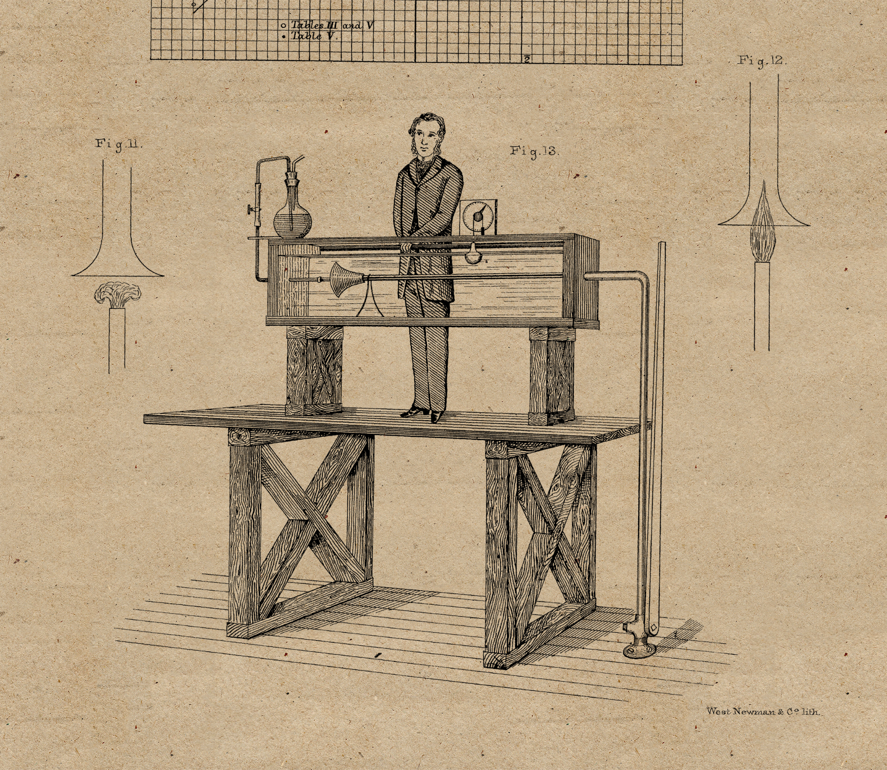
Reynolds Experiment 💧
Reynolds' investigations of the flow of fluids through tubes was published in 1883 (Reynolds, 1883). He showed most effectively that the characteristics of the flow vary with the flow velocity, and demonstrated the features of laminar and turbulent flow.
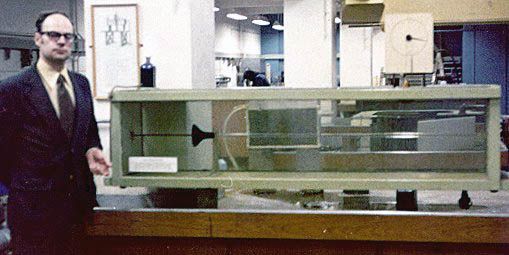
Reynolds passed water through a pipe at different flow velocities and introduced dye into the tubes to visualise fluid flow behaviour. His apparatus was very simple as can be seen in the illustration below and consisted of a glass-sided tank, 6 feet long, 18 inches deep and 18 inches wide
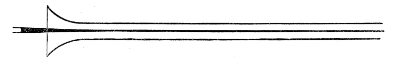
Inside the tank was a glass tube with 'a trumpet mouth of varnished wood, great care being taken to make the surface of the wood continuous with that of the glass' so that water could be injected with minimal disturbances.
On one side, the tube was connected to an iron pipe equipped with a valve which could be controlled by means of a long lever. On the other was the device for introducing a streak of dye into the trumpet. A float connected to a pulley and dial arrangement was used to register the water-level in the tank and hence the volume being discharged through the glass tube
Experiment 1️⃣
When the velocities were sufficiently low, the streak of colour extended in a beautiful straight line through the tube.
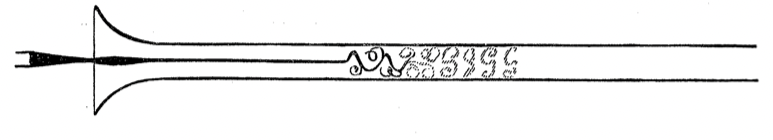
Experiment 2️⃣
At sufficiently low velocities, the streak would shift about the tube, but there was no appearance of sinuosity.
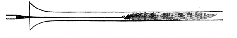
Experiment 3️⃣
As the velocity was increased by small stages, at some point in the tube, always at a considerable distance from the trumpet or intake, the colour band would all at once mix up with the surrounding water, and fill the rest of the tube with a mass of coloured water - this is turbulent flow, showing its diffusive behaviour and causing the dye to spread out.
Read more about the experiment in the original publication by Osborne Reynolds named "An Experimental Investigation of the Circumstances which determine whether the Motion of Water shall be Direct or Sinuous, and of the Law of Resistance in Parallel Channels."
Critical Reynolds Number ⚡
After this experiment, Reynolds tried to find the critical condition for an eddying flow to revert into a non-turbulent one as the flow rate is reduced, referring to this as the 'inferior limit'. To do this, he used equipment which allowed water to flow in a disturbed state from the mains supply through a length of pipe and measured the pressure-drop over a five-foot length near the outlet
The Reynolds number at which the flow becomes turbulent is called the critical Reynolds number. The value of the critical Reynolds number is different for different geometries and is a highly complicated process, which is not yet fully understood.
- For flow over a flat plate, the generally accepted value of the critical Reynolds number is Rex ≈ 500000.
- For flow in a pipe of diameter D, experimental observations show that for “fully developed” flow, laminar flow occurs when ReD < 2300, and turbulent flow occurs when ReD > 3500.
- For a sphere in a fluid, the characteristic length-scale is the sphere’s diameter, and the characteristic velocity is that of the sphere relative to the fluid. Purely laminar flow only exists up to Re = 10 under this definition.
It should be noted that the value of about 2,300 often quoted for the critical Reynolds Number is only applicable to flow in pipes, and has no relevance to other flow phenomena that depend on a Reynolds number! For instance, the Reynolds Number for water in open channels is about 6,000, and for the flow of air across a plane wing it may be from ≈50,000 upwards. As mentioned earlier, for flow in pipes and tubes engineers take the diameter as the "characteristic length measurement" (reference length).
Important Note ⚠️
I have seen a ton of students making the mistake to assume that the critical Reynolds Number is the same for every type of flow and every obstacle, which is incorrect!
The critical Reynolds Number for a pipe flow for example are not fix and can be delayed up to a Re of 50,000 or even up to 100,000 depending on the conditions without the flow becoming turbulent. The initial critical Reynolds Number found by Reynolds in his experiment for example cannot be reproduced at the same facility today as cars and trucks cause vibration in the ground that trigger a transition into a turbulent state even before the magic threshold of Re = 2,300.
Note that you will often hear that turbulent flows are special and laminar flow is the exception where it is the other way around.
Turbulence is the law, laminar is the special case.
Reynolds Number Examples👇
- A large whale swimming at 10 m/s 👉 Re = 300,000,000
- A duck flying at 20 m/s 👉 Re = 300,000
- Blood flow in the aorta 👉 Re = 1,000
- Blood flow in your brain 👉 Re = 100
- Flapping wings of the smallest flying insect 👉 Re = 30
- A bacterium swimming at 0,01 mm/s 👉 Re = 0,00001
High values of the Reynolds Number on the order of ≈10 million indicate that viscous forces are small (not negligible) and the flow is essentially inviscid. In this case, one can invoke the Euler equations to model the flow. On the other hand, low Reynolds Numbers indicate that viscous forces play an important role and must be considered.
Reynolds' Law of Similarity ✅
If you are investigating two geometrically similar flows, they are both equal to each other as long as they embrace the same Reynolds Number according to Reynolds' Law of Similarity.
Example: If you're in the wind tunnel and investigate the flow around a vehicle, you would need to have twice the speed inside the wind tunnel in order to make up for the half-scale model. Mathematically, this would look as follows:
\[ Re_{full} = \frac{\rho VD}{\mu} \]
\[ Re_{half} = \frac{\rho \mathbf{2V} \mathbf{\frac{1}{2}D}}{\mu} \]
Applications of the Reynolds Number👇
The Reynolds number plays an important part in fluid dynamics and heat transfer problems calculations.
- For the Darcy-Weisbach equation for example, it is essential to calculate the friction factor in a few of the equations of fluid mechanics. It relates the loss of pressure or head loss due to friction along the given length of pipe to the average velocity of the fluid flow for an incompressible fluid
- It is used to predict the transition from laminar to turbulent flow and in the scaling of similar but different-sized flow situations, such as between an aircraft model in a wind tunnel and the full-size version.
- The predictions of the onset of turbulence and the ability to calculate scaling effects can be used to help predict fluid behavior on a larger scale, such as in local or global air or water movement, and thereby the associated meteorological and climatological effects.
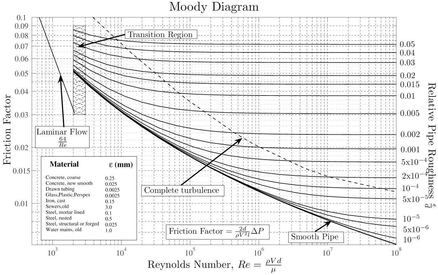
The Moody Diagram 📊
The Moody Chart (or Moody Diagram) is a diagram used in the calculation of pressure drop or head loss due to friction in pipe flow and is used to find the friction factor for flow in a pipe.
The plot shows the friction factor plotted over the Reynolds Number and relative roughness. Relative roughness is defined as the pipe roughness height, ε (epsilon), divided by the inside diameter, D. Once the Reynolds Number and relative roughness are known, the friction factor can be found from the chart and used in the Darcy-Weisbach equation for calculating the pressures loss caused by friction.
That's all folks! If you’d like to see more Fluid Mechanics blogs like this one, consider subscribing to my latest blogs, tutorials and course updates - and please feel free to leave a comment down below! 🙂
Keep engineering your mind! ❤️
Jousef