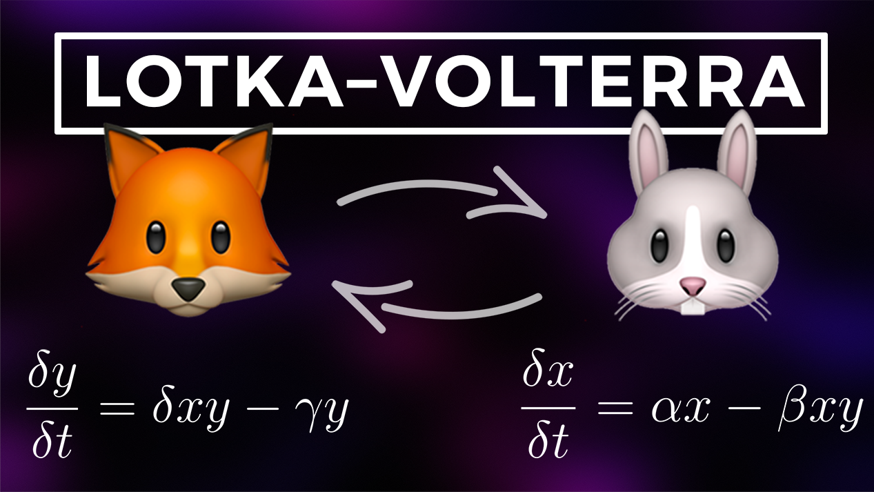
Introduction👇

The Lotka-Volterra equations were developed to describe the dynamics of biological systems. The equations can be written simply as a system of first-order non-linear ordinary differential equations (ODEs). Since the equations are differential in nature, the solutions are deterministic (no randomness is involved, and the same initial conditions will produce the same outcome), and the time is continuous (the generations of predators and prey are continually overlapping). As with many other mathematical models, many assumptions were made in the creation of the Lotka-Volterra equations.

History ⌛

The Lotka-Volterra model is the simplest model of predator-prey interactions and model was developed independently by Alfred Lotka (1925) and Vito Volterra (1926).

The model was initially proposed by Alfred Lotka in the theory of autocatalytic chemical reactions in 1910. In 1925 he used the equations to analyse predator-prey interactions in his book on biomathematics. The same set of equations was published in 1926 by Vito Volterra, a mathematician and physicist, who had become interested in mathematical biology.

Definition 📝

🦊 Predator: A predator is an organism that hunts, kills and eats other organisms to survive.

🐰 Rabbit: The prey is an organism which gets hunted and taken as food by the predator.

Assumptions 🤔

1. There is no shortage of food for the prey population
2. The food supply of the predator population depends entirely on the size of the prey population
3. The rate of change of population is directly proportional to its size
4. The environment is constant and genetic adaptation is not assumed to be negligible
5. Predators have limitless appetite

Equations 🧮

You'll often see the equation in different forms. I will demonstrate two forms so that you get a more holistic overview of the available equations.

The first version👇

Prey Equation

\[ \frac{\delta x}{\delta t} = \alpha x - \beta xy \]

• The prey are assumed to have an unlimited food supply and to reproduce exponentially (unless subject to predation)
• This exponential growth is represented in the equation above by the term 𝜶𝒙
• The rate of predation upon the prey is assumed to be proportional to the rate at which the predators and the prey meet, this is represented above by 𝜷𝒙𝒚
• If either 𝒙 or 𝒚 is zero, then there can be no predation

Predator Equation

\[ \frac{\delta y}{\delta t} = \delta xy - \gamma y \]

• In this equation, 𝜹𝒙𝒚 represents the growth of the predator population
• This is very similar to the predation rate but a different constant is used, as the rate at which the predator population grows is not necessarily equal to the rate at which it consumes the prey
• 𝜸𝒚 represents the loss rate of the predators due to either natural death or emigration, it leads to an exponential decay in the absence of prey

where:

• x is the number of prey
• y is the number of the predators
• the left side of the predator & prey equation represent the instantaneous growth rates of the two populations
• t represents the time
• α, β, γ, δ are positive real parameters describing the interaction of the two species

The second version👇

Prey Equation

\[ \dot{f}(t) = -d \cdot f(t) + c2 \cdot r(t) \cdot f(t) \]

Predator Equation

\[ \dot{r}(t) = b \cdot r(t) - c1 \cdot r(t) \cdot f(t) \]

where:

• r(t) is the population of prey (rabbits)
• f(t) is the population of predators (foxes)
• b is the birth rate of the rabbits
• d is the death rate of the foxes
• c1 is the catch rate of the rabbits
• c2 is the nutrition rate of the foxes
• r0 the initial population of rabbits
• f0 the initial population of foxes

Solution of the Model 💻

Solution in MATLAB

clear all, close all, clc

alpha = 8.5;    % Death Rate of Foxes
beta  = 10;     % Reproduction Rate of Rabbits
gamma = 0.01;   % Offspring Rate of Foxes (Thanks to Prey)
delta = 0.07;   % Death Rate of Rabbits (Through Predators)

time_start = 0;     % Starting Time
time_end = 5;     % End Time
delta_t = 1/1000;    % Time Step Increment

t  = time_start:delta_t:time_end;
nt = length(t); % Number of Time Steps

%% Initial Conditions

fox(1) = 100;
rabbit(1) = 1000;

%% 

fox(nt) = 0;
rabbit(nt) = 0;

for m = 2:nt
    fox(m) = fox(m-1) -delta_t*alpha*fox(m-1) + tau*gamma*fox(m-1)*rabbit(m-1);
    rabbit(m) = rabbit(m-1) +delta_t*beta *rabbit(m-1) - delta_t*delta*fox(m-1)*rabbit(m-1);
end

%% Plot Results

yyaxis left
plot(t,fox,'-k')
ylabel('Foxes')
hold on

yyaxis right
plot(t,rabbit,'--r')
ylabel('Rabbits')
legend('Foxes','Rabbits')

ax = gca;
ax.YAxis(1).Color = 'k';
ax.YAxis(2).Color = 'r';

title('Lotka-Volterra Equations');
xlabel('Time');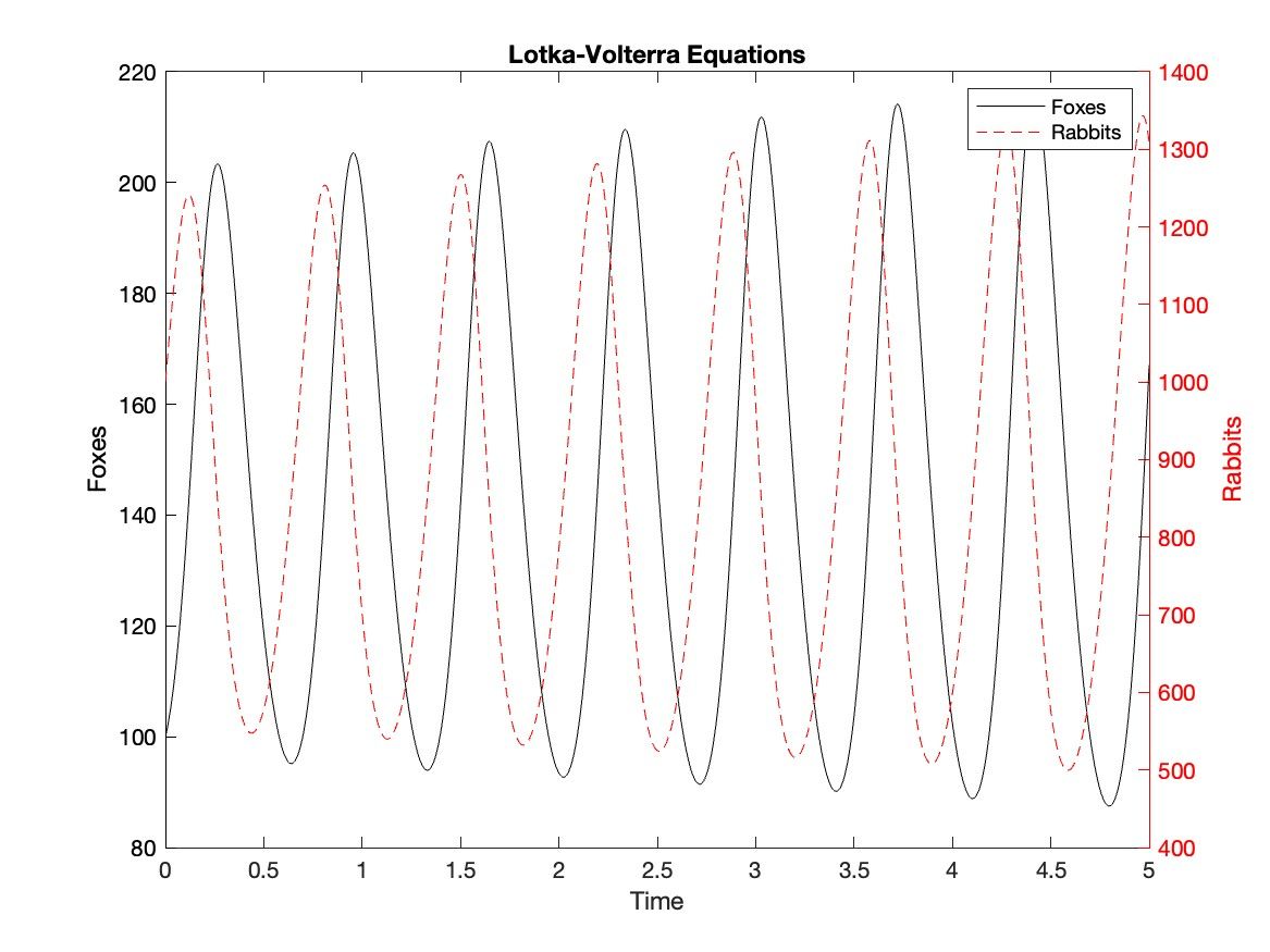

Solution in Simulink

The solution in Simulink with different parameters. The full Simulink model can be downloaded inside the MATLAB & Simulink Course.

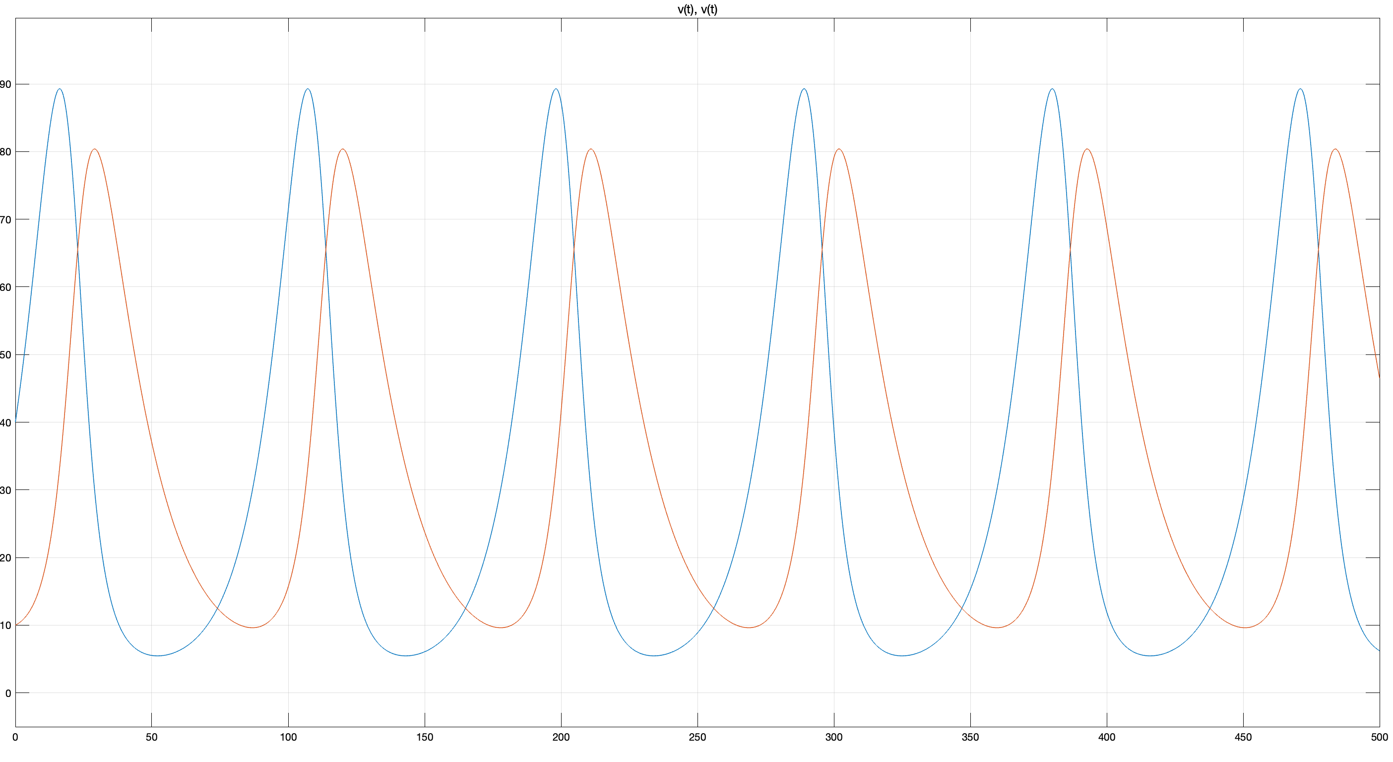
Reference Solution

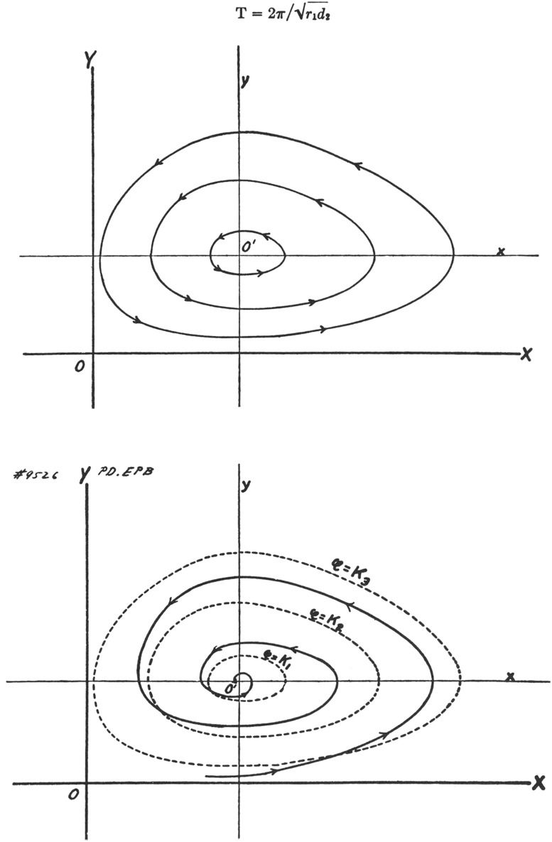
Equilibrium Conditions ⚖️

In nature, two populations can be in equilibrium with one another. To solve that with our model, the Lotka-Volterra equations, we can simply determine this equilibrium by setting the left-hand side to zero, which means nothing else than Since equilibrium means that the populations are not changing with respect to time the system of equations can be written as.

\[ 0 = \alpha x - \beta xy \]

\[ 0 = \delta xy - \gamma y \]

Drawbacks of the Model ⚡

• The probably biggest problem of the Lotka-Volterra equations is the ability of the prey population to jump back up even when the population of the prey is extremely low. The logical consequence of the model would be that the prey would go extinct at some point also causing the predators to go extinct
• The model assumes an exponential decay which would result in prey being over 100, 1000 or even 10,000 years old

If this post was helpful to you, consider subscribing to receive the latest blogs, tutorials and course updates! 🙂

And if you would love to see other blog posts or tutorials on simulation or coding, please leave a comment under this post - cheers!

Keep engineering your mind! ❤️

Jousef